Deep neural network with infinite width
To study the infinite width of neural network is of interest because of two main reasons. The first one is that the neural networks applied in the real application usually have a large width so they may share similar properties as neural networks with inifinite width. The other reason is that the neural networks with inifinite width usually have explicit properties that is easy to study. Here we try to introduce the result about the initial distribution of deep neural network with inifinite width from Jaehoon Lee etc. In this result, the initial output of the deep neural network with inifinite width will become a Gaussian Process with a kernel having a compositional structure.
Structure of Deep Neural Network
Given input \(x\in \mathbb{R}^d\), the deep neural network with \(L\) hidden layers can be expressed as the following.
\[z_i^l(x)=b_i^l+\sum_{j=1}^{N_l}W_{ij}^lx_{j}^l(x),~~~~~ x_j^l(x)=\phi(z_j^{l-1}(x))~~~~~~~ l=1,...,L\]where \(\phi(\cdot)\) is the non-linear activation such as \(tanh\) or $ReLU$.
Deep Neural Network with Infinite width
We can first derive the distribution of the output for one layer and then extend to multiple layers.
\[\newline\newline\]Single Layer Case
Now we consider the deep neural network with only 1-layer. Given the bias \(b_i^0\sim_{i.i.d}N(0,\sigma_b^2)\) and weight \(W_{ij}^0 \sim_{i.i.d} N(0,\frac{\sigma_w^2}{d})\), then we could have
\[z_i^0(x)\sim_{i.i.d} N(0, \sigma_b^2+\sigma_w^2 \frac{||x||^2}{d})~~~~ i=1,...,N_1\]And we have \(x_i^1 = \phi(z_i^0(x))\) are i.i.d.(Independent and identical distributed). Given \(b^1 \sim N(0,\sigma_b^2)\) and \(W_{i}^1\sim N(0,\frac{\sigma_w^2}{N_1})\)
Then with central limit theorem, we have
\[lim_{N_1\rightarrow \infty} z^1(x) = b^1 + W_{i}^1 x_i^1(x) \sim N(0, \sigma_b^2 + \sigma_w^2 K^0(x,x))\]Where \(K^0(x,x^\prime)=E_{z_1^0(x)}[\phi(z_1^0(x))\phi(z_1^0(x^\prime))]\).
For the covariance between \(z^1(x)\) and \(z^1(x^\prime)\). we have
\[lim_{N_1\rightarrow \infty} cov(z^1(x), z^1(x^\prime)) = \sigma_b^2 + \sigma_w^2 K^1(x,x) = K^1(x,x^\prime)\]That is, with single layer case, the initial output \(\{z^1(x)\}\) will have be a Gaussian process with kernel \(K^1(\cdot,\cdot)\).
\[\newline\newline\]Multiple Layers Case
For \(L>1\), given the initialization of bias \(b_i^l\sim N(0,\sigma_b^2) ~~ i=0,...,L\) and weights \(W_{ij}^l\sim N(0,\frac{\sigma_w^2}{N^{l}}) ~~ i=0,...,L\),we can define the compositional kernel. That is,
\[K^0(x,x^\prime)=\frac{<x,x^\prime>}{d} \newline K^l(x,x^\prime)=\sigma_b^2 + \sigma_w^2 K^{l-1}(x,x^\prime) ~~~~ l=1,...,L\]It can be proved that the for the deep neural network with \(L\) hidden layer and with the initialization illustrated as above, we could have the initial output \(\{z^L(x)\}\) will be a Gaussian process with kernel \(K^L(\cdot, \cdot)\).
\[\newline\newline\]Bayesian Inference with Deep Neural Network Kernel
Let the dataset be \(D=\lbrace x^i,t^i\rbrace_{i=1,...,n}\). Further assume that \(t^i \vert z^L(x^i)\sim N(0,\sigma_\epsilon^2)\). Then given a new data point \(x^*\), we have
\[z^* \vert D, x \sim N(\bar{\mu}, \bar{\sigma}^2)\] \[\bar{\mu} = K_{x^\*, D}(K_{D,D}+\sigma_\epsilon^2 I_n)^{-1}t\] \[\bar{\sigma}^2 = K_{x^\*,x^\*} - K_{x^\*, D}(K_{D,D}+\sigma_\epsilon^2 I_n)^{-1}K_{x^\*, D}^T\]So that we can make a prediction with Bayesian Inference.
Numerical Study
The numerical study will based on doing the bayesian inference with deep neural network kernel on the data set MNIST and CIFAR10.
Compare with the Neural Network with finite width
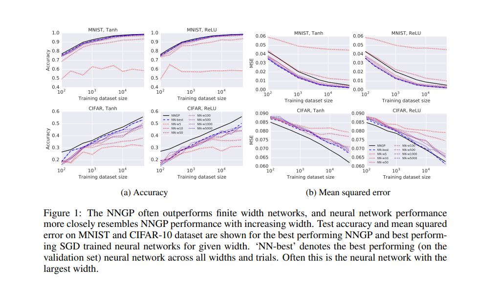
Then we have the results as below:

We can observe that the results of bayesian inference with deep neural network kernel often outperforms the neural network with finite width. Moreover, the wider the neural network, the results will be closer to the bayesian inference with deep neural network kernel.