Low rank Anova model

To model the multivariate function, One concept is the additive model.

And extended from additive modeling, functional analysis-of-variance modeling can help us to capture not only the main effect but also multi-way interaction effect of the covariates.

One issue for ANOVA modeling is the number of parameters grows exponentially as the number of covariates grows. Suppose we use the a set of spline basics with p elements, typically we will fit the interaction term by a linear combination of the tensor product basics based on the spline basics. Then there will be k power of p parameters for the k-way interaction term.

To address this problem, we assume that the multi-way interaction term has a low rank structure and we propose the low rank ANOVA modeling as shown in the formula. Suppose there are 3 covariates. The multi-way interaction term can be expressed as a product of 1-dimsional function of the covariates, By doing so, we can reduce the parameters significantly. For a set of spline basics with p elements, the number of parameters for 3-way interaction term will reduced to p*3 instead of cubic of p for the traditional ANOVA modeling.

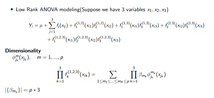
To help selecting the spline basics and interaction terms, we introduce the total variation penalty and the empirical norm penalty. With the truncated power basics, the total variation of the m-1 order derivation can be reformed as lasso penalty. So that the total variation will achieve sparse selection of knots. The empirical norm can be reformed as the L2 penalty composite with a linear transformation. And the empirical norm will help us achieve selection of interaction term.

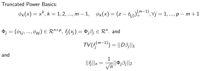
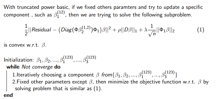
For a certain spline basic with p elements, the low rank ANOVA model can be express as formula (1). Where the star operator here represents the Hadamard product. The Phis are design matrix decide by the spline basic we choose and beta are parameters we try to fit. If we do the lease square, the loss function is not convex with respect to the whole set of parameters.

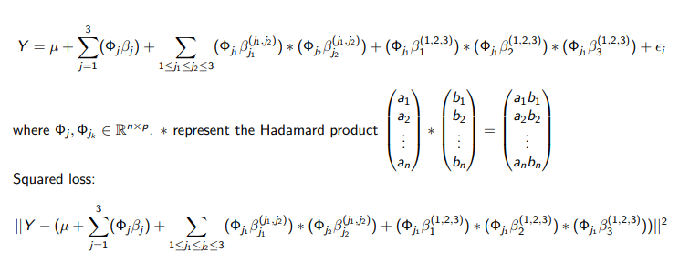
Fortunately, the loss function is convex with respect to a specific component of beta if we fixed the other. If we apply the truncated power basic and apply the total variation and empirical norm penalty , now we are trying to update the component of x1 from the interaction effect between x1 and x2, then we actually try to solve the problem as formula (2). This is a convex problem with respect to beta and actually a double penalized lease square problem. So we can apply the alternating penalized lease square scheme to fit the model. That is, we iteratively choose a component from the components set, and then we update the chosen component but make other components fixed, that is we try to solve a subproblem similar as formula (2) in each iteration.

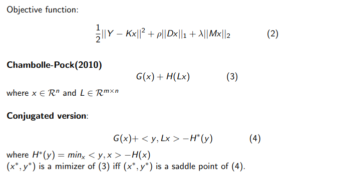
Now we discuss how to solve the double penalized least square problem we just mentioned. The subproblem can be generally formulate as equation (3). To solve the subproblem, we introduce the chambolle-pock algorithm which is a kind of primal-dual method. The objective of the algorithm is to minimize the sum of two convex function and one of them is composited with a linear transformation. Rewrite the H(Lx) in the conjugated form we have the formular as (5). And x star y star is a minimizer of (4) if and only if x star and y star is a saddle point of (5). The chambolle-pock algorithm is trying to find the saddle point of (5).

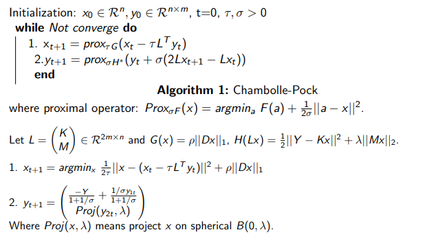
The chambolle-pock algorithm is shown here. It actually apply the proximal operator iteratively on the function G and H star to update x and y. And The proximal operator is defined as a minimization problem with a squared distance regularization. Then we can apply the chambolle-pock algorithm to solve the sub-problem in our setting. As we now can solve the sub-problem in each iteraction, then we can apply the alternating penalized least square to fit the model.

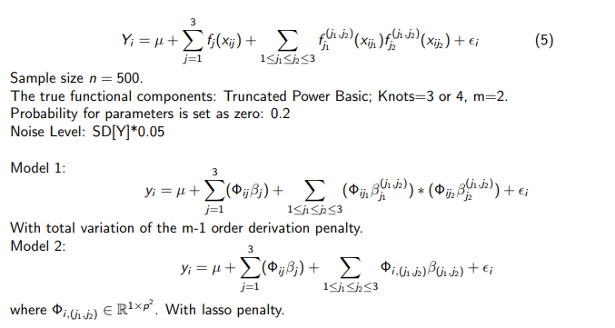
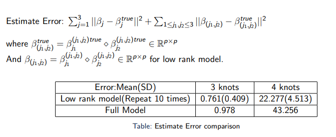
Then we will show some preliminary numerical results of the model. The simulation setting are as follow. The sample size is 500 and there will be 3 variables, the true model is the low rank ANOVA model with up to 2-way interaction. The true functional components are linear combinations of the truncated power basics with 3 or 4 knots and m = 2, which means the functional components are piece-wise linear function. To introduce the sparsity, there is a probability of 0.2 that the parameters entries to be set as 0. The noise level is 5% of the standard deviation of the response. And we will compare two model, the first one is the low rank ANOVA model with up to 2-way interaction. The second model is the full ANOVA model, that is the interaction term is assumed to be a linear combination of tensor product basics. To handle the entries-wise sparsity, we will apply the total variation penalty for model 1 and lasso penalty for model 2. The hyper-parameters for the penalty are selected by Cross-validation.

The comparison criteria is straight-forward and we just compare the squared distance between the estimate parameters and true parameters. And the table show the results. As the low rank ANOVA model problem is not convex and the alternating methods may find the local minimizers so we will repeat 10 times and report the mean and standard deviation of the estimate error for the low rank ANOVA model. From the table we can see the low rank model have a slight advantage over the full model when there is number of knots is 3 and have a significant advantage when the number of knots is 4.

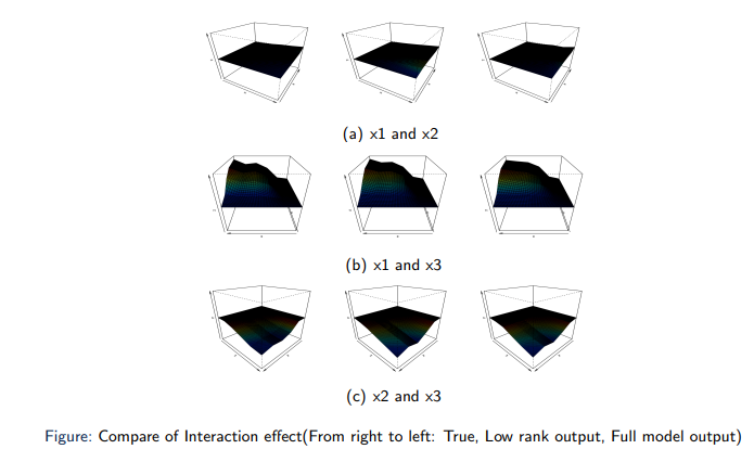
Then we try to have a more straight-forward view of the interaction effect. We can see both the estimator from the Low rank model, which is in the middle column and estimator from the full model which is in the right column can capture the main feature of the interaction effect. And Low rank model can capture more detailed feature as we can see in the interaction effect between x1 and x3. These results show that the low rank ANOVA model can have some advantage over the full ANOVA model if the true model do have a low rank structure.